Code
from dataclasses import dataclass
import torch
import torch.nn as nn
import torch.nn.functional as FIf you’ve called from transformers import BertModel or prompted GPT-4, you’ve used a Transformer. But what actually happens when it processes text? Why does attention use three separate projections: Q, K, and V? Why does the decoder need a causal mask?
The Transformer displaced a decade of sequence modelling research not because it was more complex, but because it was more general: the same architecture, with minimal changes, now handles text, images, protein structures, and audio. Understanding why it generalises is what separates someone who can use these models from someone who can reason about them.
This post builds one from scratch, understanding the motivation behind every design choice before any code. By the end, you will be able to:
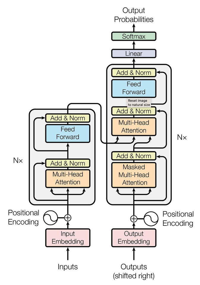
We start with the problem that motivated the Transformer (sequential bottlenecks in RNNs), build the attention mechanism from scratch, implement each component in PyTorch with annotated shapes, and assemble all three architecture variants, using the architecture diagram below as our map throughout.
To understand why the Transformer is designed the way it is, you first need to understand what it replaced, and what was fundamentally broken about it.
A Recurrent Neural Network processes a sequence one token at a time. After seeing each token \(w_t\), it updates a fixed-size hidden state \(h_t\) that is supposed to summarize everything the model has seen so far:
\[h_t = f(h_{t-1},\, w_t)\]
The hidden state is then passed to the next step. Think of it as a single notepad that a reader carries through a book, rewriting one paragraph of notes after each page. By the time they reach page 500, that notepad contains almost nothing from page 1: there simply wasn’t room to preserve it through 499 rewrites.
This is not a metaphor for a failure mode; it is the fundamental architectural constraint. The RNN must compress all prior context into a fixed-size vector, and that compression is lossy by design.
Language is full of dependencies that span many tokens. Consider:
“The trophy didn’t fit in the suitcase because it was too large.”
To resolve what “it” refers to, a model must connect a pronoun near the end of the sentence back to a noun near the beginning. In an RNN, that connection must survive through every intermediate hidden state update. Each update potentially overwrites or dilutes the earlier information. The longer the sequence, the worse this gets.
The training-time failure mirrors the inference-time failure. When we backpropagate through an RNN, the gradient of the loss with respect to early hidden states is a product of Jacobians, one per time step:
\[\frac{\partial L}{\partial h_0} = \frac{\partial L}{\partial h_T} \prod_{t=1}^{T} \frac{\partial h_t}{\partial h_{t-1}}\]
If the entries of those Jacobians are consistently less than 1 (common with bounded activations like tanh), the product shrinks exponentially with \(T\). Gradients from the loss signal barely reach the early time steps, so the model cannot learn from long-range dependencies even if it wanted to.
LSTMs and GRUs mitigate this with gating mechanisms, but they don’t eliminate it; they just slow the decay. (For a full treatment of LSTMs and their gating solution, see the Inside LSTMs post.)
RNNs are inherently sequential: you cannot compute \(h_t\) until you have \(h_{t-1}\). This makes it impossible to parallelize across the time dimension. For a sequence of length \(T\), the forward pass requires \(T\) sequential steps regardless of how many GPUs you have.
Modern GPUs are massively parallel processors: they shine on matrix multiplications that can be batched across thousands of operations simultaneously. RNNs waste almost all of that capacity.
RNNs fail in three compounding ways: (1) the hidden state bottleneck loses information over long sequences; (2) vanishing gradients prevent learning long-range relationships from the training signal; (3) sequential computation prevents parallelization, making training slow regardless of hardware. The Transformer addresses all three, not with patches, but by replacing sequential recurrence with a fundamentally different mechanism.
The central insight of the Transformer is deceptively simple: throw out sequential processing entirely and let every token communicate directly with every other token, in a single parallel operation.
With an RNN, every relationship between tokens must be mediated through the hidden state. Information travels through a long chain before it reaches its destination. With attention, every token asks every other token directly: “How relevant are you to me?” The answer shapes what information each token receives.
This is a fundamentally different computational paradigm: instead of routing information through a bottleneck, we create a direct, differentiable communication channel between all pairs of tokens simultaneously. The attention matrix for a sequence of length \(T\) is \(T \times T\). Every pair gets its own weight.
The attention mechanism is most naturally understood as a soft database lookup.
Imagine walking into a library. You have a query in mind: say, you’re looking for books about long-range dependencies in sequences. Every book in the library has a key on its spine: a short descriptor of what’s inside. You compare your query against every key, computing a relevance score for each book. Then you retrieve the values (the actual content) weighted by those relevance scores. The most relevant books contribute the most to what you walk away knowing.
This is exactly what the Transformer’s attention mechanism does at every layer, for every token:
The attended output for each token is a weighted mixture of all value vectors, where the weights are determined by the similarity between that token’s query and all other tokens’ keys.
Attention is not a neural network layer in the traditional sense; it is a soft, differentiable database lookup. It is differentiable because the retrieval weights are produced by a smooth function (softmax), so gradients flow through the lookup operation during backpropagation. The queries, keys, and values are all learned: the model learns what to look for, what to advertise, and what to say.
We’ll return to this library analogy throughout: it explains why Q, K, and V need to be separate projections, and what the attention weights actually represent numerically.
Here is the deeper insight that explains why Vision Transformers, AlphaFold2, audio Transformers, and point cloud Transformers all use the same architecture as BERT and GPT, often with almost no modification.
The Transformer has almost no structural inductive bias. CNNs assume that nearby pixels are related: they bake in locality and translation equivariance as a prior. RNNs assume sequential order: they process left-to-right by construction. The Transformer assumes nothing about the structure of its input beyond what the positional encoding tells it. Every pair of positions is treated symmetrically by the attention mechanism until the training data says otherwise.
This is simultaneously the weakness and the superpower:
The key insight: positional encoding is the only thing that changes across domains. The attention mechanism, FFN, LayerNorm, and residual connections are entirely domain-agnostic. Swap the positional encoding and the same architecture processes any structured data. This is why the Transformer became the universal architecture, not because it is uniquely suited to language, but because it is uniquely generic.
Before anything else, raw text must be converted into numbers that the model can process. This conversion (tokenization) splits text into a vocabulary of subword units and maps each unit to an integer ID. The Transformer receives a B × T matrix of integers as input, where B is the batch size and T is the sequence length.
There are three families of tokenization strategy (character-level, word-level, and subword), each with distinct tradeoffs in vocabulary size, sequence length, and out-of-vocabulary handling. Modern language models universally use subword tokenization (BPE or WordPiece), which offers a vocabulary of tens of thousands of tokens while gracefully handling rare and novel words by decomposing them into known pieces.
This post focuses on the Transformer architecture that consumes tokenized sequences, not on tokenization itself. For a deep dive into how tokenization works:
The embedding layer is the first thing the model does with the token IDs it receives. It has two jobs: turn integers into meaningful vectors, and inject positional information so the model knows where each token sits in the sequence.
An integer ID has no geometric structure. The number 42 is not “close to” 41 in any meaningful sense for language. The token at position 42 in the vocabulary might be completely unrelated to token 41. Neural networks need continuous-valued vectors they can do math on: compute dot products, measure distances, apply linear transformations.
A token embedding is a lookup table: a matrix of shape vocab_sz × embed_dim where each row is a learnable vector associated with one token. When the model sees token ID \(i\), it looks up row \(i\) and uses that vector downstream.
What makes embeddings powerful is that training forces semantically similar tokens into nearby regions of this vector space. After training on enough text, the embedding for “king” minus the embedding for “man” plus the embedding for “woman” lands close to “queen”, not because we encoded this relationship by hand, but because the training signal shaped the space that way.
An embedding turns a name tag into a GPS coordinate: suddenly you can measure distance, find neighbors, and do arithmetic.
Shape: B × T (integer IDs) → B × T × embed_dim (float vectors)
Weight tying. In most language models, the embedding matrix is reused as the output projection at the end of the network: the final linear layer that maps from d_model back to vocab_sz uses the same weights, transposed. This is called weight tying. The core intuition: if two tokens have similar embeddings (i.e., they are semantically close), they should also receive similar probabilities when the model generates the next-token distribution. Since the LM head scores each candidate token by taking the dot product of the model’s output vector with that token’s embedding row, tokens whose embedding vectors are close to the output vector will score similarly, producing nearby probabilities. Weight tying enforces this consistency directly: the same geometry that groups similar tokens together in the input space also determines their relative scores in the output distribution. As a bonus, it halves the parameter count for the vocabulary components (often 30–100K tokens × 768 dims = a significant share of total parameters) and keeps input and output representations aligned throughout training.
Word order is one of the primary mechanisms through which human languages encode meaning. Consider how much information is carried purely by where a word sits in a sentence:
Order determines who does what to whom. “The dog bit the man” and “The man bit the dog” contain identical tokens. The meaning is completely reversed. Without positional information, a model sees the same set of embeddings for both; it cannot distinguish them.
Agreement and dependency span long distances. In “The cats that live in the house are noisy”, the verb “are” must agree with “cats” (plural), not “house” (singular). Correctly resolving this requires knowing that “cats” appears before the relative clause, and “house” is inside it, a structural relationship determined entirely by position.
Negation scope is positional. “I never said she stole the money” and “I said she never stole the money” contain the same words. The position of “never” determines the scope of negation: whether the speaker denies making the claim or denies the theft itself.
Modifier attachment is determined by proximity. “I photographed the man with a telescope” is ambiguous in isolation. In context, positional proximity to either “man” or “photographed” is the primary cue for whether the telescope was used for photographing or was held by the man.
In short: token embeddings capture what each word means in isolation; positional encodings capture where each word sits, which encodes its grammatical role, its relationships to surrounding words, and its structural function in the sentence.
Here is the technical issue: attention is permutation equivariant. If you reorder the input tokens, the output tokens reorder identically: the attention mechanism has no internal sense of sequence order. From the model’s perspective, “the cat sat on the mat” and “the mat sat on the cat” produce the same set of output vectors (just shuffled). Position is invisible.
To fix this, we add positional encodings to the token embeddings before feeding them into the Transformer. The result: two otherwise identical tokens at different positions get different combined representations, making order visible to every downstream layer.
There are three main strategies:
The original Transformer paper uses fixed, non-learned positional encodings based on sine and cosine functions at different frequencies:
\[PE_{(pos,\, 2i)} = \sin\!\left(\frac{pos}{10000^{2i/d}}\right)\] \[PE_{(pos,\, 2i+1)} = \cos\!\left(\frac{pos}{10000^{2i/d}}\right)\]
Why low dimensions oscillate fast and high dimensions oscillate slowly comes directly from the formula. The denominator \(10000^{2i/d}\) is the key: it grows exponentially with the dimension index \(i\). Dividing by a larger number slows the wave down:
| Dimension \(i\) | Denominator \(10000^{2i/d}\) | Wave period (positions for one full cycle) | What it encodes |
|---|---|---|---|
| \(i = 0\) | \(1\) | ~6 positions | Very fine: distinguishes adjacent tokens |
| \(i = d/8\) | \(\approx 18\) | ~110 positions | Phrase-level distance |
| \(i = d/4\) | \(\approx 316\) | ~2,000 positions | Sentence-level distance |
| \(i = d/2\) | \(10{,}000\) | ~62,800 positions | Barely changes: encodes very coarse, document-level position |
Think of it as an odometer: the rightmost digit (low dimension) flips every meter, the leftmost digit (high dimension) barely moves over a typical journey. Each digit alone is ambiguous: the rightmost digit of “7” could be position 7, 17, 27, or 107. But all digits together uniquely identify every position.
This multi-scale design is intentional. Low dimensions give the model a fine-grained signal that changes every few positions, useful for detecting whether two tokens are immediate neighbors. High dimensions give a coarse signal that changes only over long distances, useful for detecting whether two tokens are in the same half of the document. Together, the full vector is unique for every position from 0 to the maximum.
The advantage of sinusoidal encodings is that they can generalize to sequence lengths longer than those seen during training: the functions extend naturally to any position.
Instead of fixing the positional encoding by formula, we can make it a learned parameter: another nn.Embedding table of shape max_seq_len × embed_dim. Each position from 0 to max_seq_len-1 gets its own learnable row, updated via backpropagation just like token embeddings.
This is what BERT and GPT use. The model learns what positional fingerprints work best for its task. The downside: sequences longer than max_seq_len seen during training have no positional encoding; the model has never learned what those positions mean.
RoPE, introduced by Su et al. (2021) and used in LLaMA, Mistral, and GPT-NeoX, takes a fundamentally different approach: instead of adding a fixed vector to the embeddings, it rotates the query and key vectors by an angle proportional to their absolute position before computing the attention dot product.
The key property: when you rotate \(Q\) at position \(m\) and \(K\) at position \(n\), their dot product becomes a function of only the relative distance \(m - n\):
\[Q_m \cdot K_n = f(m - n)\]
This is highly desirable. Relative position (how far apart two tokens are) is often more informative than absolute position. Whether “cat” is token 5 or token 50 in the sentence matters less than how far it sits from the verb it modifies. Syntactic dependencies (subject → verb, adjective → noun) tend to hold over short distances regardless of where the sentence begins. RoPE bakes this directly into the attention computation at every layer, without requiring separate positional embedding vectors.
RoPE also generalizes better to longer sequences than the model was trained on, making it the dominant choice in modern open-source LLMs.
The code below uses learned absolute positional embeddings, the simplest approach and standard for BERT-style encoder models. The embedding layer adds the token embedding and positional embedding, normalizes with LayerNorm, and applies dropout.
from dataclasses import dataclass
import torch
import torch.nn as nn
import torch.nn.functional as F@dataclass
class TransformerConfig:
vocab_sz: int = 1000
block_sz: int = 8
hidden_dropout_prob: float = 0.2
num_attention_heads: int = 12
num_hidden_layers: int = 6
embed_dim: int = 768
num_classes: int = 2
layer_norm_eps: float = 1e-12
intermediate_sz: int = 0 # set to 4 * embed_dim in __post_init__
def __post_init__(self):
if self.intermediate_sz == 0:
self.intermediate_sz = 4 * self.embed_dim
config = TransformerConfig()class Embeddings(nn.Module):
def __init__(self, config):
super().__init__()
self.token_embedding = nn.Embedding(config.vocab_sz, config.embed_dim)
self.position_embedding = nn.Embedding(config.block_sz, config.embed_dim)
self.layer_norm = nn.LayerNorm(config.embed_dim, eps=config.layer_norm_eps)
self.dropout = nn.Dropout(p=0.1)
def forward(self, x):
## x: B x T (integer token IDs)
## token_emb: B x T x embed_dim
## position_emb: T x embed_dim (broadcast over batch)
## output: B x T x embed_dim
seq_len = x.shape[1]
positions = torch.arange(seq_len, device=x.device)
embeddings = self.token_embedding(x) + self.position_embedding(positions)
embeddings = self.layer_norm(embeddings)
return self.dropout(embeddings)import numpy as np
import matplotlib.pyplot as plt
import matplotlib
matplotlib.rcParams["figure.dpi"] = 150
def sinusoidal_pe(seq_len, d_model):
pe = np.zeros((seq_len, d_model))
pos = np.arange(seq_len)[:, None]
i = np.arange(d_model)[None, :]
div = 10000 ** (2 * (i // 2) / d_model)
pe[:, 0::2] = np.sin(pos / div[:, 0::2])
pe[:, 1::2] = np.cos(pos / div[:, 1::2])
return pe
pe = sinusoidal_pe(seq_len=64, d_model=128)
fig, ax = plt.subplots(figsize=(10, 3.5))
img = ax.imshow(pe.T, cmap="RdBu_r", aspect="auto", vmin=-1, vmax=1)
ax.set_xlabel("Position in sequence", fontsize=12)
ax.set_ylabel("Embedding dimension", fontsize=12)
ax.set_title(
"Sinusoidal Positional Encoding: each column is a unique position fingerprint",
fontsize=11, pad=8
)
plt.colorbar(img, ax=ax, fraction=0.015, pad=0.02, label="Encoding value")
plt.tight_layout()
plt.savefig("positional-encoding-heatmap.png", dpi=150, bbox_inches="tight")
plt.show()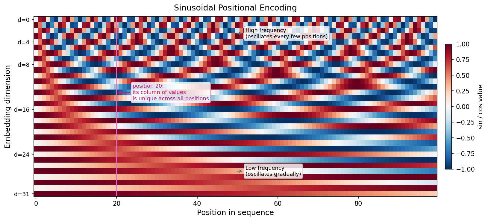
Attention is the core computation that makes everything else in the Transformer work. Everything up to this point (embeddings, positional encodings) has been preprocessing. This is the operation that enables direct token-to-token communication.
This section builds it up step by step: from the Q/K/V projections, through the dot-product similarity, scaling, softmax, and masking. By the end, the library analogy from Section 2 will have a precise mathematical form.
Given an input sequence \(x\) of shape B × T × embed_dim, we produce three separate linear projections:
\[Q = xW_Q, \quad K = xW_K, \quad V = xW_V\]
Each weight matrix (\(W_Q\), \(W_K\), \(W_V\)) has shape embed_dim × head_dim. These are learned parameters: different projection matrices produce different “perspectives” on the same input.
Why three separate projections instead of one? Because what a token wants (its query), what it offers to match against (its key), and what it actually communicates (its value) are three genuinely different things. Consider how a search engine works: your search query text (Q) is compared against the indexed keywords of a web page (K), but what you actually receive when you click is the full page content (V), which may be organized completely differently from the index terms. Separating these three roles gives the model the flexibility to learn very different relationships for each.
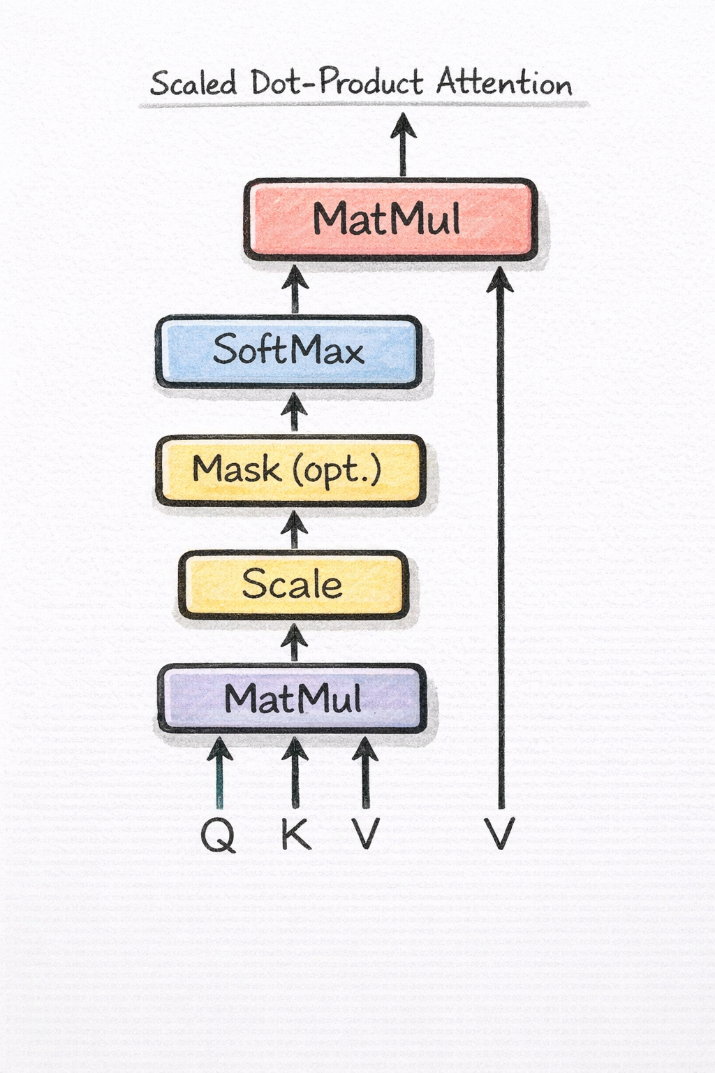
With Q, K, V in hand, the attention weights are computed as:
\[\text{weights} = \text{softmax}\!\left(\frac{QK^T}{\sqrt{d_k}}\right)\]
Let’s trace through this with a concrete 3-token example. Suppose our sequence is [“the”, “cat”, “sat”], with head_dim = 4. After the Q and K projections, imagine we have:
\[Q = \begin{bmatrix} 1 & 0 & 1 & 0 \\ 0 & 1 & 0 & 1 \\ 1 & 1 & 0 & 0 \end{bmatrix},\quad K = \begin{bmatrix} 1 & 0 & 0 & 1 \\ 0 & 1 & 1 & 0 \\ 1 & 1 & 0 & 0 \end{bmatrix}\]
Step 1. Dot products \(QK^T\) (shape 3 × 3): Every token’s query is dotted with every token’s key. The \((i,j)\) entry measures how much token \(i\) “wants” to attend to token \(j\).
\[QK^T = \begin{bmatrix} 1 & 1 & 2 \\ 1 & 1 & 0 \\ 1 & 2 & 2 \end{bmatrix}\]
Why dot products? Geometrically, the dot product of two vectors is large when they point in similar directions (small angle) and small when they are orthogonal. If a query and key are aligned (the token is “looking for” exactly what the other token “offers”), the dot product is high, and that token will receive a large attention weight.
Step 2. Scale by \(\frac{1}{\sqrt{d_k}} = \frac{1}{2}\):
\[\frac{QK^T}{\sqrt{d_k}} = \begin{bmatrix} 0.5 & 0.5 & 1.0 \\ 0.5 & 0.5 & 0.0 \\ 0.5 & 1.0 & 1.0 \end{bmatrix}\]
Step 3. Softmax row-wise (each row sums to 1):
\[\text{weights} = \begin{bmatrix} 0.27 & 0.27 & 0.46 \\ 0.33 & 0.33 & 0.33 \\ 0.21 & 0.39 & 0.39 \end{bmatrix}\]
Row 1 (token “the”): attends most strongly to “sat” (0.46). Row 2 (“cat”): distributes evenly. Row 3 (“sat”): attends most to “cat” and itself.
![Figure 3: Attention weights for the [‘the’, ‘cat’, ‘sat’] example. Rows are query tokens; columns are keys. Each row is a probability distribution: how much each token attends to every other token.](images/attention-weights-matrix.png)
Step 4. Multiply by V (shape 3 × head_dim): The output for each token is a weighted combination of all value vectors, with weights from the softmax step. Token “the” will receive a mix of all three value vectors, weighted 27%/27%/46%. The output is a contextualized representation: the same token in a different sentence would produce different weights and therefore a different output vector.
Notice what just happened: the token “the”, which starts with a fixed embedding vector identical in every sentence, now has a representation shaped by the presence of “cat” and “sat.” Run the same token through a different sentence (“the table broke”), and it emerges from attention with a different output vector.
This is the fundamental departure from static word embeddings like word2vec or GloVe: those give every token a single, context-free vector that never changes. A Transformer gives every token a contextual representation, numerically different depending on what surrounds it. “bank” in “river bank” and “bank” in “bank account” start with the same embedding but diverge after attention. This is why Transformer-based representations are so dramatically better at tasks requiring word sense disambiguation, coreference resolution, and syntactic parsing.
This is one of those design choices that looks arbitrary until you understand the numerical reason behind it.
Q and K are both initialized as approximately unit-variance random vectors. When you compute their dot product across d_k dimensions, the result has variance equal to \(d_k\) (sum of d_k independent unit-variance terms). For a typical head_dim of 64, the raw dot products have standard deviation 8. For head_dim = 768, standard deviation 27.
Large-magnitude inputs to softmax cause a saturation problem. When one logit is much larger than the others, softmax approaches a one-hot distribution: almost all weight goes to one token, and gradients for every other position become negligibly small. The model can only learn from the one token it attends to, and ignores all the rest.
Dividing by \(\sqrt{d_k}\) rescales the dot products back to approximately unit variance, regardless of head_dim. Softmax then produces a diffuse distribution (not too concentrated, not too uniform), and gradients flow to all positions during training.
Without scaling, attention becomes a dictatorship: one token captures all the weight and the rest are ignored. Scaling preserves the democracy: every token can contribute to the output.
Why use softmax and not sigmoid (or any other normalization)?
Sigmoid applied to each attention logit independently would allow a token to “attend highly to everyone” at the same time, with no trade-off. But attention should be selective: attending more to one token means attending less to others.
Softmax is a competitive normalization: its outputs sum to 1, so the weights form a probability distribution over the context window. Increasing attention to one token necessarily decreases attention to all others. This forces the model to make decisions about what is relevant rather than attending indiscriminately to everything.
The exponential creates sparsity, not just competition. Softmax uses \(e^x\), not a simple linear normalization like dividing by the sum. The exponential amplifies differences: if one logit is 2 points higher than another, it receives \(e^2 \approx 7\times\) more weight, not just 2× more. In practice this means attention patterns are often peaky: a small number of tokens receive the vast majority of the weight, and the rest are nearly zero. This emergent sparsity is what makes attention heads interpretable: a head that attends sharply to the syntactic subject has learned a crisp, readable pattern, not a diffuse smear. It also means that a single highly-relevant token can dominate the output almost entirely, which is the mechanism behind induction heads and other sharp attention circuits found in mechanistic interpretability research.
In a language model, the task is to predict the next token from all previous tokens. If the model can see token \(t+1\) while predicting token \(t\), that is data leakage: the model would just copy the future token rather than learning to predict it.
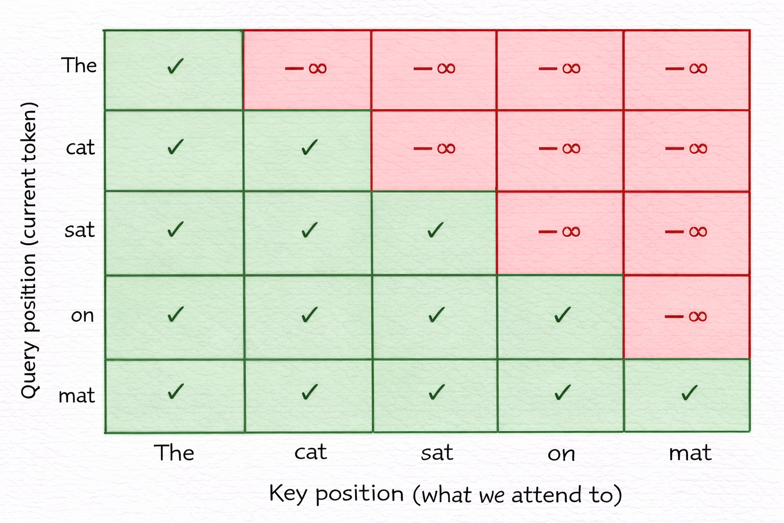
After softmax, \(-\infty\) becomes exactly 0. Token 1 can only attend to itself. Token 3 can attend to tokens 1, 2, and 3 but not 4. The mask enforces a strict information asymmetry: you can read anything in the past, but nothing in the future.
This is implemented by registering a lower-triangular buffer in the AttentionHead and calling masked_fill before softmax.
Self-attention: Q, K, and V all come from the same input sequence \(x\). Every token attends to every other token within the same sequence. This is what the encoder uses (bidirectional) and the decoder uses for its first sublayer (causal).
Cross-attention: Q comes from one sequence (the decoder’s hidden state), while K and V come from a different sequence (the encoder’s output). The decoder “reads” the encoder’s representation of the source sequence. This is the mechanism that connects the two halves of an encoder-decoder model.
The generalization is worth stating explicitly: any two sequences can be related through cross-attention, simply by using one as the source of Q and the other as the source of K and V. This is the same operation that connects modalities in vision-language models (text queries attend to image patch keys/values), that lets perceiver architectures compress long inputs (a small set of learned query vectors attends to a large input), and that underlies virtually all multi-modal conditioning. Cross-attention is not a feature of encoder-decoder models; it is a universal conditioning primitive.
The full attention equation:
\[\text{Attention}(Q, K, V) = \text{softmax}\!\left(\frac{QK^T}{\sqrt{d_k}}\right)V\]
Computing attention requires forming the full \(T \times T\) weight matrix: every token’s query dotted against every token’s key. This is \(O(T^2 \cdot d_k)\) time and \(O(T^2)\) memory. For most sentences this is fine. For long documents, it becomes the dominant constraint:
| Sequence length | Attention matrix | Memory (fp16, 1 head) |
|---|---|---|
| 512 tokens | 512 × 512 = 262K | ~0.5 MB |
| 4,096 tokens | 4K × 4K = 16.8M | ~32 MB |
| 128K tokens | 128K × 128K = 16.4B | ~31 GB |
This quadratic growth is why early BERT was capped at 512 tokens, why getting GPT-3 to handle long documents required tricks, and why an entire subfield of efficient attention exists: sliding-window attention (Longformer), linear attention, sparse attention (BigBird), and state-space models like Mamba are all attempts to approximate or restructure the \(T \times T\) computation to grow linearly with sequence length.
FlashAttention (Dao et al., 2022) is often described as “making attention faster.” What it actually does: reorders the computation to tile through the attention matrix in blocks that fit in GPU SRAM (fast memory), avoiding slow round-trips to HBM (GPU global memory). The FLOPs are identical to standard attention; the memory bandwidth cost drops dramatically: 2–4× wall-clock speedup with numerically identical outputs. It also reduces peak memory from \(O(T^2)\) to \(O(T)\) by never materializing the full attention matrix. This is why FlashAttention is the standard in every modern training stack, but it does not fix the fundamental quadratic scaling problem for very long contexts.
class AttentionHead(nn.Module):
    def __init__(self, config, head_dim, is_decoder=False) -> None:
        super().__init__()
        self.q = nn.Linear(config.embed_dim, head_dim, bias=False)
        self.k = nn.Linear(config.embed_dim, head_dim, bias=False)
        self.v = nn.Linear(config.embed_dim, head_dim, bias=False)
        self.is_decoder = is_decoder
        if self.is_decoder:
            self.register_buffer(
                "mask", torch.tril(torch.ones(config.block_sz, config.block_sz))
            )

    def forward(self, query, key, value):
        ## query: B x T_q x embed_dim  (source of queries)
        ## key:   B x T_k x embed_dim  (source of keys)
        ## value: B x T_k x embed_dim  (source of values)
        q = self.q(query)  ## B x T_q x head_dim
        k = self.k(key)    ## B x T_k x head_dim
        v = self.v(value)  ## B x T_k x head_dim
        ## w: B x T_q x T_k  (pairwise similarity between every query and every key)
        w = q @ k.transpose(2, 1) / (k.shape[-1] ** 0.5)
        if self.is_decoder:
            T = w.shape[-1]
            w = w.masked_fill(self.mask[:T, :T] == 0, -float("inf"))
        w = F.softmax(w, dim=-1)
        ## output: B x T_q x head_dim
return w @ vA single attention head learns one type of relationship between tokens. For example, it might learn to focus on the syntactic subject of a sentence whenever any token is processed, a subject-finding head. But language has many simultaneous relationship types that are all relevant at once:
Multiple heads allow the model to learn all of these in parallel. Each head has its own independent weight matrices \(W_Q^h\), \(W_K^h\), \(W_V^h\) that project the same input \(x\) into a different lower-dimensional subspace:
\[\text{head\_dim} = \frac{\text{embed\_dim}}{\text{num\_heads}}\]
This subspace separation is the mechanism that makes specialization both possible and stable. Head 3’s attention weights are determined by \(W_Q^3 \cdot W_K^3\) inner products, which have nothing to do with what \(W_Q^7 \cdot W_K^7\) computes for head 7. Because they project into orthogonal subspaces of the embedding, heads don’t interfere with each other: a coreference head and a subject-finding head can coexist without one corrupting the other.
Empirical findings from BERTology (Clark et al., 2019) confirm that this specialization emerges after training: some heads consistently track syntactic dependencies across the entire network; others attend primarily to adjacent tokens, effectively implementing a local sliding window; some heads in BERT-style models attend heavily to the [SEP] token, a kind of “no-op” head that routes excess attention somewhere harmless when no strong relationship exists.
Importantly, this specialization is not designed in. It arises entirely from the training signal. The architecture only provides the capacity for parallel, independent subspace projections; training discovers what each subspace should track.
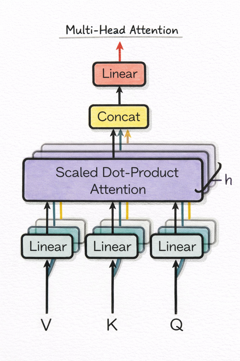
Each head produces an output of shape B × T × head_dim. All heads run entirely in parallel: there is no communication between heads during the forward pass. The outputs of all heads are concatenated along the last dimension: num_heads × head_dim = embed_dim. The concatenated tensor then passes through a final linear projection \(W_O\) of shape embed_dim × embed_dim.
Why the final projection? The heads operated in isolation: each found something different in its own subspace. The \(W_O\) projection is the first opportunity for the model to mix information across heads: to combine what the coreference head found with what the subject-finding head found into a single coherent output vector. But \(W_O\) does more than concatenate: it filters and compresses. The 12 concatenated head outputs may contain redundant information, conflicting signals, or noise from heads that found nothing relevant. \(W_O\) is a learned projection that selects which cross-head combinations to amplify and which to suppress. Think of it as the editor who takes 12 reporters’ raw notes and synthesises them into a single coherent paragraph; not every detail makes it through.
The implementation below uses a Python loop over heads for clarity. In practice, all heads are computed in a single batched matrix multiply by reshaping the input to B × T × num_heads × head_dim and transposing. This is the approach used in production (and in torch.nn.MultiheadAttention). The pedagogical loop is equivalent but slower.
However, there is still a problem: multi-head attention is a weighted averaging operation; it is linear in V. Stacking multiple attention layers with nothing in between collapses to a single linear transformation. The network needs nonlinearity. That is the feed-forward network’s job.
class MultiHeadAttention(nn.Module):
    def __init__(self, config, is_decoder=False) -> None:
        super().__init__()
        head_dim = config.embed_dim // config.num_attention_heads
        self.heads = nn.ModuleList(
            [
                AttentionHead(config, head_dim, is_decoder)
                for _ in range(config.num_attention_heads)
            ]
        )
        ## Final projection mixes information across heads: embed_dim -> embed_dim
        self.output_proj = nn.Linear(config.embed_dim, config.embed_dim)

    def forward(self, query, key, value):
        ## query: B x T_q x embed_dim
        ## key:   B x T_k x embed_dim
        ## value: B x T_k x embed_dim
        ## Each head produces B x T_q x head_dim; cat gives B x T_q x embed_dim
        x = torch.cat([head(query, key, value) for head in self.heads], dim=-1)
return self.output_proj(x) ## B x T_q x embed_dimAttention is a weighted averaging operation. It is linear in V: the output for each position is a linear combination of value vectors, where the combination weights come from the attention scores. If we stacked multiple attention layers with no nonlinearity in between, the composition of linear operations would remain linear, effectively equivalent to a single layer.
This is the same reason we use activation functions between layers in any neural network: without them, depth buys us nothing.
The feed-forward network (FFN) adds the essential nonlinearity. It processes each token’s representation independently after the attention layer. There is no mixing of tokens in the FFN; that is attention’s job. The clean separation of concerns is intentional:
The FFN as a knowledge store. Research by Geva et al. (2021) provides a compelling interpretation: FFN layers function as associative memories. The first linear layer acts as a set of keys that pattern-match against the input; the second linear layer acts as the corresponding values that are retrieved and output. Most of a Transformer’s factual knowledge (the associations between entities, relations, and attributes) is hypothesized to live in FFN weights, not in the attention matrices.
Attention is the routing system. The FFN is the knowledge store.
The FFN has a characteristic structure: expand, activate, contract.
embed_dim → 4 × embed_dim. The 4x factor is empirical, found to work well across a range of model sizes. The expanded intermediate dimension is where most of the model’s representational capacity lives, and it is the dimension that is typically scaled up when making larger models.4 × embed_dim → embed_dim, restoring the original dimension for the residual connection.Why position-wise? The FFN applies the same learned transformation to every position independently and in parallel. There is no weight-sharing across positions within a layer, but the same weight matrices process every position. This is sometimes called a “position-wise” or “point-wise” feed-forward layer.
Most of the parameters live here. Each attention layer has four weight matrices (Q, K, V, O), each of size \(d_{\text{model}} \times d_{\text{model}}\), totalling \(4d_{\text{model}}^2\) parameters. The FFN has two matrices of size \(d_{\text{model}} \times 4d_{\text{model}}\), totalling \(8d_{\text{model}}^2\) parameters: twice as many as attention. Across a full model, the FFN accounts for roughly two-thirds of all trainable parameters. When people talk about “scaling” a Transformer, they mostly mean growing \(d_{\text{model}}\) and \(d_{\text{ff}}\), which expands this majority share.
class FeedForwardNN(nn.Module):
    def __init__(self, config):
        super().__init__()
        ## Expand to 4x hidden dim, then contract back; most capacity lives here
        self.l1 = nn.Linear(config.embed_dim, config.intermediate_sz)
        self.l2 = nn.Linear(config.intermediate_sz, config.embed_dim)
        self.dropout = nn.Dropout(config.hidden_dropout_prob)

    def forward(self, x):
        ## x:        B x T x embed_dim
        ## after l1: B x T x intermediate_sz  (expand)
        ## after l2: B x T x embed_dim        (contract)
return self.dropout(self.l2(F.gelu(self.l1(x))))Deep networks have a training stability problem: as signals propagate through many layers, the distribution of activations tends to shift and grow, a phenomenon called internal covariate shift. Layers that receive wildly varying input distributions must constantly adjust their weights just to track the shifting scale, not to learn meaningful transformations. This wastes capacity and slows training.
Think of it as keeping the working range of each layer consistent. Without normalization, earlier layers can produce outputs 100x larger than what later layers expect: the later layers waste capacity on a bookkeeping problem rather than learning anything about language.
Normalization is the engineering fix: explicitly constrain activation distributions to zero mean and unit variance at key points in the network, keeping signals in a regime where gradients are well-behaved throughout training.
Batch Normalization (Ioffe & Szegedy, 2015) normalizes each feature across the batch dimension. This works well for CNNs on images but has two critical failure modes for sequence models:
Layer Normalization (Ba et al., 2016) normalizes across the feature dimension instead of the batch dimension:
\[y = \frac{x - \mathbb{E}[x]}{\sqrt{\text{Var}[x] + \epsilon}} \cdot \gamma + \beta\]
The mean and variance are computed independently for each example, over all features of that example. This makes LayerNorm completely independent of batch size: it works identically whether batch size is 1 or 1000.
| Batch Norm | Layer Norm | |
|---|---|---|
| Normalizes over | Batch dimension | Feature dimension |
| Running statistics for inference | Yes | No |
| Breaks for batch_size = 1 | Yes | No |
| Variable-length sequences | Awkward | Natural |
| Common in | CNNs, image models | Transformers, RNNs |
The learnable parameters \(\gamma\) and \(\beta\): After normalization, every layer’s output would have zero mean and unit variance, too rigid. The learned scale (\(\gamma\)) and shift (\(\beta\)) let each layer restore whatever distribution works best for its downstream computation. Without them, normalization would over-constrain the model.
The original Transformer paper placed LayerNorm after the residual addition (Post-LayerNorm). GPT-2 and virtually every modern large model places it before (Pre-LayerNorm). This seemingly minor change has significant consequences for training stability.
graph LR
    subgraph PostLN["Post-LN (original paper)"]
        A1[x] --> B1[Sublayer]
        A1 --> C1[+]
        B1 --> C1
        C1 --> D1[LayerNorm]
        D1 --> E1[output]
    end
    subgraph PreLN["Pre-LN (GPT-2, modern default)"]
        A2[x] --> B2[LayerNorm]
        B2 --> C2[Sublayer]
        A2 --> D2[+]
        C2 --> D2
        D2 --> E2[output]
    end
Post-LN: LN(x + sublayer(x)) |
Pre-LN: x + sublayer(LN(x)) |
|
|---|---|---|
| Gradient path | Normalization sits outside the residual (gradients must pass through it) | Normalization is inside (clean gradient highway through the residual) |
| Training stability | Sensitive; requires careful learning rate warm-up; can diverge | More stable; trains without warm-up |
| Final performance | Marginally better with enough tuning | Slightly lower ceiling, but much easier to train |
Modern practice defaults to Pre-LN: training stability at scale is worth more than marginal final performance differences. If you are building a new model, use Pre-LN.
Think of a Transformer as a residual stream: a river of information that flows from the input through all the layers to the output. Each layer (attention + FFN) reads from the stream and writes a correction back to it via addition:
\[x_{\text{out}} = x_{\text{in}} + \text{sublayer}(x_{\text{in}})\]
No single layer “owns” the representation. Each layer adds its contribution to a shared river. The residual stream at any point contains the sum of everything all previous layers have written.
This framing, developed in mechanistic interpretability research, makes it immediately clear why attention heads can specialize: each head contributes independently and additively to the stream. They don’t compete or overwrite each other; they contribute independently, and the stream accumulates all contributions.
Gradient highways. When backpropagating through \(y = x + F(x)\):
\[\frac{\partial L}{\partial x} = \frac{\partial L}{\partial y} \cdot \left(1 + \frac{\partial F}{\partial x}\right)\]
The term \(\frac{\partial L}{\partial y}\) reaches \(x\) directly, through the identity path, regardless of what \(F(x)\) does. Even if \(F\) has saturated activations or near-zero gradients, the loss signal still flows back to earlier layers. This is why ResNets with skip connections can be trained to hundreds of layers while the same architecture without them fails beyond a dozen.
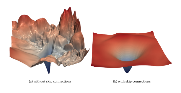
Loss landscape smoothing. He et al. (2016) visualized the loss surfaces of deep networks with and without skip connections. Without them: chaotic, sharp, with many high-curvature local minima that trap gradient descent. With them: smooth, convex, much more navigable.
The forgetting argument. Without skip connections, each layer must preserve all useful information from its input in its output: if the layer wants to pass something unchanged, it must learn to do so explicitly. With skip connections, the default is identity: the layer only needs to learn what to add, not what to keep. This dramatically reduces the effective depth that the gradient must overcome.
However, training deep networks reliably requires one more ingredient beyond gradient highways: preventing the network from memorizing noise. That is dropout’s job.
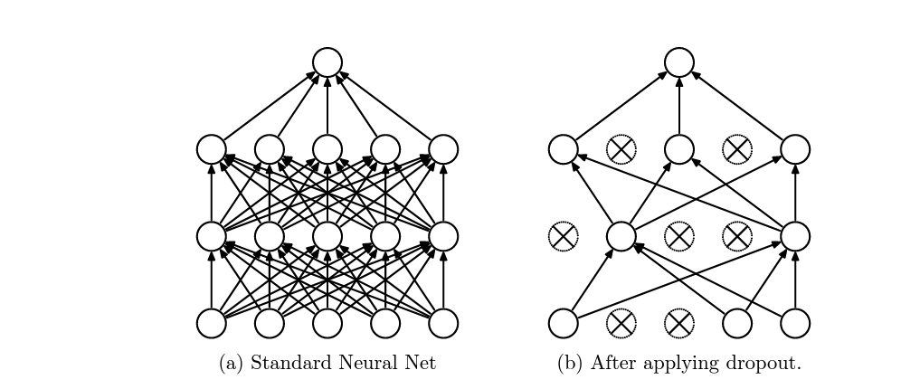
Dropout (Srivastava et al., 2014) randomly zeros a fraction p of activations during training. Each training step uses a different random mask, forcing the model not to rely on any particular activation path, a phenomenon called co-adaptation prevention.
The regularization effect comes from two mechanisms:
In Transformers, dropout is applied after the embedding layer (after adding token + positional embeddings), after each attention sublayer, and after each FFN sublayer.
LLaMA, Mistral, and other recent large models use no dropout at all. At sufficient scale with enough data, the regularization effect of dropout is less necessary, and it slows training. Dropout remains important for smaller models trained on limited data, and for fine-tuning where overfitting is a risk.
With all the individual components understood (attention, FFN, LayerNorm, skip connections, dropout), it’s time to see how they snap together into a complete layer.
Now that we have all the building blocks, let us see how they snap together into a single encoder layer: the repeated unit that makes up the encoder stack.
An encoder layer applies two sublayers in sequence, each wrapped in a residual connection and LayerNorm. Tracing the shapes at every step (using Pre-LN convention):
| Step | Operation | Shape | What it does |
|---|---|---|---|
| 1 | Input Embeddings | (B, T, d_model) |
Token IDs → dense vectors |
| 2 | + Positional Encoding | (B, T, d_model) |
Inject position information |
| 3 | Self-Attention (xh heads) | (B, T, d_model) |
Each token attends to all others |
| 4 | Add & Norm | (B, T, d_model) |
Residual connection + layer norm |
| 5 | Feed-Forward | (B, T, d_ff) → (B, T, d_model) |
Non-linear transformation |
| 6 | Add & Norm | (B, T, d_model) |
Residual connection + layer norm |
| 7 | [Repeat × N layers] | (B, T, d_model) |
Stack N encoder layers |
| 8 | Encoder Output | (B, T, d_model) |
Rich contextual representations |
B = batch size, T = sequence length, d_model = model dimension
Why every row says d_model. Residual connections require that the sublayer output has exactly the same shape as its input; otherwise you cannot add them together. This is a hard architectural constraint: every sublayer (attention, FFN, LayerNorm) must consume and produce tensors of shape (B, T, d_model). It is the reason head_dim = d_model / num_heads (the concatenation of all heads must restore d_model), and why the FFN contracts back from d_ff → d_model at the end. The entire Transformer is shaped around this single number.
Every token’s representation enters with shape d_model. After the attention sublayer, it has been updated by attending to all other tokens: information has been mixed across positions. After the FFN sublayer, each position’s representation has been transformed nonlinearly, independently from all other positions.
An encoder layer does two things: (1) let tokens talk to each other via attention, then (2) let each token digest what it heard via the FFN.
A full encoder stacks \(N\) of these layers (typically 6–24). Each layer refines the representations further: early layers tend to capture surface-level patterns, later layers capture increasingly abstract semantic relationships.
The implementation below uses the Post-LayerNorm arrangement from the original paper: LN(x + sublayer(x)). The Pre-LN alternative is shown in comments. For new models, prefer Pre-LN.
class EncoderLayer(nn.Module):
    def __init__(self, config):
        super().__init__()
        self.attn = MultiHeadAttention(config)
        self.ff = FeedForwardNN(config)
        self.layer_norm_1 = nn.LayerNorm(config.embed_dim)
        self.layer_norm_2 = nn.LayerNorm(config.embed_dim)

    def forward(self, x):
        ## x: B x T x embed_dim  (input and output shape are identical)
        ##
        ## Post-LayerNorm arrangement (original Transformer paper):
        x = self.layer_norm_1(x + self.attn(x, x, x))  ## bidirectional self-attention
        x = self.layer_norm_2(x + self.ff(x))
        ##
        ## Pre-LayerNorm alternative (GPT-2+, more stable, recommended for new models):
        ## x = x + self.attn(self.layer_norm_1(x), self.layer_norm_1(x), self.layer_norm_1(x))
        ## x = x + self.ff(self.layer_norm_2(x))
        return x  ## B x T x embed_dim
class TransformerEncoder(nn.Module):
def __init__(self, config) -> None:
super().__init__()
self.embeddings = Embeddings(config)
self.encoder_blocks = nn.Sequential(
*[EncoderLayer(config) for _ in range(config.num_hidden_layers)]
)
def forward(self, x):
## x: B x T (integer token IDs)
x = self.embeddings(x) ## B x T x embed_dim
return self.encoder_blocks(x) ## B x T x embed_dimThe decoder layer differs from the encoder in one critical way: it adds a cross-attention sublayer between the masked self-attention and the FFN. This is the mechanism that lets the decoder read the encoder’s output.
A decoder layer applies three sublayers:
| Step | Operation | Shape | What it does |
|---|---|---|---|
| 1 | Target Embeddings | (B, T_tgt, d_model) |
Target token IDs → dense vectors |
| 2 | + Positional Encoding | (B, T_tgt, d_model) |
Inject position information |
| 3 | Masked Self-Attention (xh) | (B, T_tgt, d_model) |
Attends only to past positions (causal mask) |
| 4 | Add & Norm | (B, T_tgt, d_model) |
Residual connection + layer norm |
| 5 | Cross-Attention (×h) | (B, T_tgt, d_model) |
Q from decoder; K, V from encoder output |
| 6 | Add & Norm | (B, T_tgt, d_model) |
Residual connection + layer norm |
| 7 | Feed-Forward | (B, T_tgt, d_ff) → (B, T_tgt, d_model) |
Non-linear transformation |
| 8 | Add & Norm | (B, T_tgt, d_model) |
Residual connection + layer norm |
| 9 | [Repeat × N layers] | (B, T_tgt, d_model) |
Stack N decoder layers |
| 10 | Linear + Softmax | (B, T_tgt, vocab_size) |
Project to vocabulary probabilities |
B = batch size, T_tgt = target sequence length
Sublayer 1 (masked self-attention): Decoder tokens attend to each other, but only to past and current positions (causal mask). This builds a contextualized representation of the target sequence generated so far.
Sublayer 2 (cross-attention): The decoder’s hidden state becomes the query. The encoder’s final output provides the keys and values. Every decoder position can attend to all encoder positions: this is how the decoder “reads” the full source sequence at every generation step.
Sublayer 3 (FFN): Same position-wise transformation as in the encoder.
The DecoderLayer shown uses only masked self-attention (no cross-attention sublayer). It is therefore suited for the decoder-only (GPT-style) architecture. Cross-attention is addressed in the Encoder-Decoder section.
class DecoderLayer(nn.Module):
    def __init__(self, config):
        super().__init__()
        self.attn = MultiHeadAttention(config, is_decoder=True)
        self.ff = FeedForwardNN(config)
        self.layer_norm_1 = nn.LayerNorm(config.embed_dim)
        self.layer_norm_2 = nn.LayerNorm(config.embed_dim)

    def forward(self, x):
        ## x: B x T x embed_dim
        ## Masked self-attention: each token only attends to past and current positions
        x = self.layer_norm_1(x + self.attn(x, x, x))
        x = self.layer_norm_2(x + self.ff(x))
        return x  ## B x T x embed_dim
class TransformerDecoder(nn.Module):
def __init__(self, config) -> None:
super().__init__()
self.embeddings = Embeddings(config)
self.decoder_blocks = nn.Sequential(
*[DecoderLayer(config) for _ in range(config.num_hidden_layers)]
)
def forward(self, x):
## x: B x T (integer token IDs)
x = self.embeddings(x) ## B x T x embed_dim
return self.decoder_blocks(x) ## B x T x embed_dimThe same building blocks support three distinct architectures, differing only in which sublayers are present and whether attention is masked. Here is the full comparison before diving into each:
| Encoder-Only | Decoder-Only | Encoder-Decoder | |
|---|---|---|---|
| Attention masking | Bidirectional | Causal | Causal in decoder; bidirectional in encoder |
| Cross-attention | No | No | Yes |
| Input → Output | Text → hidden states | Text → next token | Source text → target text |
| Canonical task | Classification, NER, embeddings | Text generation, LM | Translation, summarization |
| Examples | BERT, RoBERTa, DistilBERT | GPT, LLaMA, Mistral | T5, BART, mT5 |
Encoder-only models use bidirectional self-attention: every token attends to every other token with no masking. This means the representation of each token is conditioned on the full context: tokens to the left and the right. Bidirectional context makes encoder-only models excellent at understanding tasks: text classification, named entity recognition, extractive question answering, and computing sentence embeddings.
Why bidirectional? Classification does not require generating new tokens; it requires understanding the full input. A model that sees the entire sentence simultaneously can build richer representations than one forced to read left-to-right.
How is it trained? BERT-style models are trained with Masked Language Modeling (MLM): 15% of tokens are randomly masked ([MASK]), and the model must predict the original token at each masked position. Because the model can see all tokens to the left and right of the mask, this forces it to build bidirectional representations.
Classification head. A special [CLS] token is prepended to every sequence before the encoder. The encoder’s output at the [CLS] position (encoder_output[:, 0, :]) serves as an aggregate representation of the full sequence. This vector is passed through a linear classification head to produce logits.
BERT uses [CLS] because it is trained to aggregate sequence-level information during pretraining (next sentence prediction task). In practice, mean pooling over all token representations often performs equally well or better for downstream tasks. Modern models trained without NSP use mean pooling as the default.
class TransformerForSequenceClassification(nn.Module):
    def __init__(self, config):
        super().__init__()
        self.encoder = TransformerEncoder(config)
        self.dropout = nn.Dropout(config.hidden_dropout_prob)
        self.classifier = nn.Linear(config.embed_dim, config.num_classes)

    def forward(self, x):
        ## x:              B x T  (integer token IDs)
        ## encoder output: B x T x embed_dim
        ## [CLS] vector:   B x embed_dim  (position 0 aggregates sequence meaning)
        ## logits:         B x num_classes
        cls_output = self.encoder(x)[:, 0, :]
return self.classifier(self.dropout(cls_output))Decoder-only models use causal self-attention: each token can only attend to itself and previous tokens. This is the natural architecture for language modeling: predicting the next token given all previous tokens.
Why causal? Generating text requires predicting one token at a time. If the model could see future tokens while predicting token \(t\), it would simply copy them. The causal mask enforces the constraint that prediction at position \(t\) uses only information from positions \(0, 1, \ldots, t\).
The training objective: Causal Language Modeling (CLM). Decoder-only models are trained by next-token prediction: given a sequence of tokens, predict the next one at every position simultaneously. The loss is the average cross-entropy over all positions. Because the causal mask prevents each position from seeing future tokens, a single forward pass generates \(T\) training examples from one sequence: every position is simultaneously a training target. This is why CLM scales so efficiently: a 2048-token document yields 2048 gradient signals per forward pass. The training objective directly shapes what the model learns: because it must predict the next token from all preceding context, the model is forced to compress everything useful about the past into each position’s representation, which is why later layers hold increasingly abstract, predictive features.
Autoregressive generation. At inference, the decoder generates text by repeating:
graph LR
    A["Input tokens
[BOS, t₁, t₂]"] --> B["Decoder
(causal attention)"]
    B --> C["LM head
(linear + softmax)"]
    C --> D["Next token
t₃"]
    D --> A
vocab_sz, then softmax)Sampling strategies control how token \(t+1\) is chosen from the distribution:
KV caching: why inference is efficient. The loop as described implies re-computing attention over the full growing sequence at every step, which would scale as \(O(T^2)\) for a \(T\)-token generation. Production systems avoid this with a KV cache: the K and V tensors for all past positions are stored after their first computation and reused on every subsequent step. Only the new token’s Q needs to be computed; it attends to the cached K/V from all prior positions. Each generation step then costs \(O(T \cdot d)\) instead of \(O(T^2 \cdot d)\).
The KV cache is a first-class engineering constraint in LLM deployment. For a model with \(L\) layers, \(H\) heads, head dimension \(d_k\), and current sequence length \(T\), the cache requires \(2 \cdot L \cdot H \cdot d_k \cdot T\) values; for LLaMA-3 70B at 4K context in fp16, that is roughly 5 GB. This is precisely why Grouped Query Attention (GQA) exists: by sharing a single K/V head across multiple Q heads, the cache shrinks by a factor of num_heads / num_kv_heads, often 8x. Every major modern model (LLaMA 2/3, Mistral, Gemma) uses GQA for exactly this reason.
class GPT(nn.Module):
    def __init__(self, config):
        super().__init__()
        self.decoder = TransformerDecoder(config)
        self.dropout = nn.Dropout(config.hidden_dropout_prob)
        ## Project from embed_dim to vocab_sz to get next-token logits
        self.lm_head = nn.Linear(config.embed_dim, config.vocab_sz, bias=False)

    def forward(self, x):
        ## x:       B x T  (integer token IDs)
        ## decoded: B x T x embed_dim
        ## logits:  B x T x vocab_sz  (next-token distribution at every position)
        x = self.dropout(self.decoder(x))
        return self.lm_head(x)
class CrossAttentionDecoderLayer(nn.Module):
"""Decoder layer with three sublayers:
(1) masked causal self-attention, (2) cross-attention to encoder, (3) FFN.
"""
def __init__(self, config):
super().__init__()
self.self_attn = MultiHeadAttention(config, is_decoder=True)
self.cross_attn = MultiHeadAttention(config, is_decoder=False)
self.ff = FeedForwardNN(config)
self.layer_norm_1 = nn.LayerNorm(config.embed_dim)
self.layer_norm_2 = nn.LayerNorm(config.embed_dim)
self.layer_norm_3 = nn.LayerNorm(config.embed_dim)
def forward(self, x, encoder_output):
## x: B x T_dec x embed_dim
## encoder_output: B x T_enc x embed_dim
##
## 1. Masked self-attention: decoder tokens attend to each other causally
x = self.layer_norm_1(x + self.self_attn(x, x, x))
## 2. Cross-attention: Q from decoder, K and V from encoder
## Every decoder position can attend to all encoder positions
x = self.layer_norm_2(x + self.cross_attn(x, encoder_output, encoder_output))
## 3. Position-wise FFN
x = self.layer_norm_3(x + self.ff(x))
return x ## B x T_dec x embed_dim
class Seq2SeqTransformer(nn.Module):
"""Encoder-decoder Transformer for sequence-to-sequence tasks
such as machine translation and summarization.
"""
def __init__(self, config):
super().__init__()
self.encoder_embeddings = Embeddings(config)
self.decoder_embeddings = Embeddings(config)
self.encoder_blocks = nn.ModuleList(
[EncoderLayer(config) for _ in range(config.num_hidden_layers)]
)
self.decoder_blocks = nn.ModuleList(
[CrossAttentionDecoderLayer(config) for _ in range(config.num_hidden_layers)]
)
self.lm_head = nn.Linear(config.embed_dim, config.vocab_sz, bias=False)
def encode(self, src):
## src: B x T_enc → B x T_enc x embed_dim
x = self.encoder_embeddings(src)
for block in self.encoder_blocks:
x = block(x)
return x ## B x T_enc x embed_dim
def decode(self, tgt, encoder_output):
## tgt: B x T_dec
## encoder_output: B x T_enc x embed_dim
x = self.decoder_embeddings(tgt) ## B x T_dec x embed_dim
for block in self.decoder_blocks:
x = block(x, encoder_output)
return x ## B x T_dec x embed_dim
def forward(self, src, tgt):
## src: B x T_enc (source token IDs, e.g. English)
## tgt: B x T_dec (target token IDs, e.g. German; teacher-forced during training)
encoder_output = self.encode(src) ## B x T_enc x embed_dim
decoder_output = self.decode(tgt, encoder_output) ## B x T_dec x embed_dim
return self.lm_head(decoder_output) ## B x T_dec x vocab_szThe encoder-decoder (or “sequence-to-sequence”) architecture is the original Transformer from Vaswani et al. (2017). It is designed for tasks where both input and output are text sequences, particularly tasks where the input and output are structurally different, like machine translation or summarization.
The two-phase interpretation:
How cross-attention implements conditioning. At every decoder step, the cross-attention sublayer takes:
Every decoder position attends to all encoder positions simultaneously. The model learns which parts of the source to focus on when generating each target token: the alignment between source and target.
Note that unlike self-attention (where the \(T \times T\) weight matrix is square), cross-attention produces a rectangular weight matrix of shape \(T_{\text{tgt}} \times T_{\text{src}}\): one row per decoder query position, one column per encoder key position. During early generation when only a few target tokens exist, this matrix might be \(3 \times 50\): three decoder positions each attending over fifty source positions. The asymmetry is intentional: the decoder decides what to ask (Q), the encoder provides the full library of keys and values (K, V), and the weight matrix records what each decoder step borrows from each source position.
When encoder-decoder vs. decoder-only? Encoder-decoder models are preferred when source and target are structurally different (e.g., English → German, document → summary). For tasks where both input and output are similar in format (e.g., open-domain conversation, code completion), decoder-only models have largely taken over: they are simpler to train and scale, and can handle both input and output within a single sequence by formatting the task as a text completion problem.
Notable encoder-decoder models: T5 (Text-to-Text Transfer Transformer), BART, mT5, NLLB.
Let’s trace a complete forward pass through an encoder-decoder Transformer to see how all the pieces compose. We’ll use a small example: translating the English sentence “The cat sat” into German.
Setup: batch size \(B = 1\), source length \(T_{enc} = 3\), embed_dim = 768, num_heads = 12, head_dim = 64.
Step 1. Tokenize the source.
“The cat sat” → subword tokenizer → [2, 47, 193] (integer IDs)
Shape: 1 × 3 (integers)
Step 2. Token embedding lookup.
Each integer is mapped to a 768-dimensional vector via the embedding table.
Shape: 1 × 3 → 1 × 3 × 768
Step 3. Add positional encodings.
A positional encoding vector is added to each token’s embedding. The result encodes both what the token is (token embedding) and where it sits (positional encoding).
Shape: 1 × 3 × 768 (unchanged)
Step 4. N encoder layers.
Each encoder layer applies two sublayers:
Shape at every encoder layer: 1 × 3 × 768 (unchanged throughout)
After \(N\) encoder layers, each of the 3 token positions holds a deeply contextualized representation: the meaning of “cat” is now informed by the presence of “The” and “sat” in context.
Encoder output: 1 × 3 × 768, which is what the decoder will attend to.
Step 5. Decoder receives the start token.
Decoder input starts with a start-of-sequence token [BOS].
Shape: 1 × 1 → (after embedding) 1 × 1 × 768
Step 6. N decoder layers.
Each decoder layer applies three sublayers:
Masked self-attention: Only 1 token so far, so the \(1 × 1\) causal attention matrix is trivially “attend to self.” Shape: 1 × 1 × 768.
Cross-attention: Q comes from the decoder hidden state (1 × 1 × 768). K and V come from the encoder output (1 × 3 × 768). Attention weights have shape 1 × 1 × 3: the single decoder position attends to all 3 encoder positions. Output: 1 × 1 × 768.
FFN: 1 × 1 × 768 processed position-wise.
Step 7. LM head.
The decoder output at the final position (1 × 1 × 768) is projected to vocab_sz via a linear layer, then softmax gives a probability distribution over the vocabulary.
Shape: 1 × 1 × 768 → 1 × 1 × vocab_sz → sample token → e.g., "Die" (German “The”)
Step 8. Autoregressive loop.
Append "Die" to the decoder input. Repeat Steps 6–7 with decoder input [BOS, "Die"] to generate the next token. Continue until [EOS] is sampled or the maximum length is reached.
The key insight from this walkthrough: the encoder runs once for the full source sequence. The decoder runs once per generated token, attending to the full encoder output (which never changes) at every step via cross-attention.
Understanding the architecture is one thing; understanding what trained Transformers actually compute is another. Here is a brief map of empirical findings.
Clark et al. (2019) systematically analyzed BERT’s attention patterns across all layers and heads and found striking specialization:
[SEP] heads: Many heads in middle layers attend heavily to [SEP] tokens. The interpretation: when no strong relationship exists, these heads use [SEP] as a “garbage collector”, routing excess attention somewhere harmless.This specialization is emergent, not designed. It arises purely from the training signal on downstream tasks.
Geva et al. (2021) showed that FFN sublayers act as key-value memories. The first linear layer’s weight rows act as “keys” that activate on specific input patterns; the second linear layer’s corresponding columns act as “values” that are retrieved and output.
This framing explains where factual knowledge lives in a language model. When a model correctly completes “The Eiffel Tower is located in ___“, the relevant association (Eiffel Tower → Paris) is likely stored as a key-value pair in the FFN weights of one or more layers, not in the attention matrices.
Probing classifiers (small models trained to predict linguistic properties from internal representations) consistently find that:
The architecture explains why this gradient exists. Early layers receive representations that have undergone very little contextualization: essentially just the token and positional embeddings. They can only access local, surface-level patterns. Later layers, on the other hand, are reading from a residual stream that has already accumulated many rounds of attention and FFN processing. Each layer builds on the contextualized representations produced by all previous layers, enabling increasingly abstract structures to emerge. The depth gradient is not a design choice; it is a direct consequence of how information accumulates through residual connections.
The original Transformer (2017) has been refined substantially. Here are the key improvements that appear in modern LLMs, with brief explanations of why each was adopted:
| Improvement | What changes | Why | Used in |
|---|---|---|---|
| Pre-LayerNorm | LN moves inside the residual branch | Training stability at scale; no warm-up required | GPT-2, LLaMA, Mistral |
| Rotary Position Embedding (RoPE) | Replaces absolute pos. embeddings with rotation of Q and K | Better length generalization; relative position naturally encoded at every layer | LLaMA, Mistral, GPT-NeoX, Qwen |
| Grouped Query Attention (GQA) | Multiple Q heads share a single K and V head | Reduces KV cache memory at inference without meaningful accuracy loss | LLaMA 2/3, Mistral |
| SwiGLU activation | Replaces GELU in FFN with a gated linear unit: \(\text{SwiGLU}(x) = \text{Swish}(xW_1) \odot xW_2\) | Consistently higher benchmark performance at equivalent parameter counts | LLaMA, PaLM, Gemma |
| FlashAttention | Reorders attention computation to minimize memory bandwidth | \(O(N)\) memory instead of \(O(N^2)\); 2–4x faster; identical numerical outputs | Used in most modern training stacks |
| RMSNorm | Replaces LayerNorm with root-mean-square normalization (no mean subtraction) | Simpler, ~10% faster, equivalent quality | LLaMA, Mistral, Gemma |
In this post, we built the Transformer architecture from scratch, starting from the failure modes of RNNs, building the attention mechanism step by step, implementing each component in PyTorch with annotated shapes, and assembling the encoder-only, decoder-only, and encoder-decoder variants. We also traced a complete end-to-end forward pass and surveyed what trained Transformers empirically learn.
The architecture’s dominance across language, vision, speech, and biology stems from a coherent set of design choices, each solving a specific problem with a specific mechanism.
Attention replaces sequential recurrence with parallel direct communication. Every token attends to every other token in a single matrix operation. No hidden state bottleneck, no sequential dependency, no vanishing gradient through time: the fundamental failures of RNNs are eliminated at the architectural level, not patched over.
Q, K, V separation is intentional, not arbitrary. What a token wants (query), what it offers (key), and what it says (value) are three genuinely different roles. Separating them, as in the library lookup analogy, gives the model the flexibility to learn very different relationships for each. A single projection would conflate all three.
Multi-head attention gives the model multiple simultaneous perspectives. Each head operates in its own lower-dimensional subspace and learns to track different relationship types: one head for syntax, one for coreference, one for local context. This specialization is emergent: it arises from the training signal, not from any explicit design constraint.
The FFN is the knowledge store; attention is the routing system. Attention decides which tokens talk to which and mixes their representations. The FFN then transforms each token’s representation independently and nonlinearly: this is where factual associations are stored. Without the FFN, stacked attention layers collapse to a single linear transformation.
Skip connections and LayerNorm make depth trainable. Residual connections create gradient highways that bypass each sublayer entirely, making it possible to train networks dozens of layers deep. Pre-LayerNorm (inside the residual branch) stabilizes training at scale without requiring learning rate warm-up.
Architecture determines what tokens can see; everything else is shared. The only fundamental difference between an encoder and a decoder is the causal mask. The same attention mechanism, FFN, LayerNorm, and residual structure underlies all three variants (encoder-only, decoder-only, and encoder-decoder), differing only in which tokens each position is allowed to attend to.
Despite years of improvements (RoPE, GQA, SwiGLU, FlashAttention, RMSNorm), the fundamental architecture described in this post has not changed since 2017. The overall structure (attention + FFN + residual + norm, stacked \(N\) times) is the same in GPT-4, LLaMA 3, and Gemini as it was in the original “Attention Is All You Need.” If you understand this post, you understand the backbone of essentially all modern AI.
What to explore next: