Code
import numpy as np
import torch
import torch.nn as nn
import torch.nn.functional as FIf you’ve used nn.LSTM in PyTorch, you’ve seen it work. But how does it decide what to remember and what to forget? Why does it need four gates instead of one? And why is it so much better than a vanilla RNN at handling long sequences?
The best way to answer these questions is to build one yourself. In this post, we’ll start with the problem that motivated LSTMs (vanishing gradients), build up the intuition for how they solve it, then implement both LSTMCell and a multi-layer LSTM from scratch in PyTorch, verifying each against the official implementation down to floating-point precision.
Long Short-Term Memory (LSTM) is a recurrent neural network architecture introduced by Hochreiter and Schmidhuber (1997) to solve the vanishing gradient problem: the central failure mode of vanilla RNNs on long sequences.
To understand why LSTMs exist, we first need to understand what goes wrong. In a vanilla RNN, the hidden state is completely overwritten at every time step:
\[h_t = \tanh(W_{hh} \cdot h_{t-1} + W_{xh} \cdot x_t + b)\]
During backpropagation, the gradient of the loss with respect to an early hidden state \(h_1\) must pass through the \(\tanh\) nonlinearity and the weight matrix \(W_{hh}\) at every single time step between \(h_T\) and \(h_1\). If the sequence has 100 tokens, the gradient is multiplied by \(W_{hh}\) roughly 100 times. If the dominant eigenvalue of \(W_{hh}\) is even slightly less than 1 (say 0.9), the gradient shrinks by a factor of \(0.9^{100} \approx 0.00003\). The signal from early tokens effectively disappears.
The problem isn’t just mathematical. It has a concrete consequence: vanilla RNNs can’t learn long-range dependencies. If the answer to a question depends on a word 50 tokens earlier in the sentence, the gradient signal connecting them is essentially zero. The model can’t learn that relationship, no matter how long you train.
The LSTM introduces a cell state \(c_t\): a separate memory channel that runs parallel to the hidden state. The critical difference is in how it gets updated:
| Vanilla RNN | LSTM Cell State | |
|---|---|---|
| Update rule | \(h_t = \tanh(W \cdot h_{t-1} + \ldots)\) | \(c_t = f_t \odot c_{t-1} + i_t \odot g_t\) |
| Mechanism | Complete replacement through nonlinearity | Selective modification via additive gating |
| Gradient flow | Must pass through \(\tanh\) and \(W\) at every step | Can flow directly through the forget gate \(f_t\) |
| Long-range memory | Exponential decay | Controlled retention |
The cell state update is additive: when the forget gate \(f_t\) is close to 1 and the input gate \(i_t\) is close to 0, the cell state passes through unchanged: \(c_t \approx c_{t-1}\). Gradients flow backward through time with minimal decay: no weight matrix or nonlinearity in the way.
If this looks familiar, it should. It’s the same principle behind residual connections in ResNets. In a ResNet, each layer computes \(y = F(x) + x\): the input passes through unchanged, and the layer only learns the residual. The LSTM cell state works the same way, but across time instead of depth: the previous cell state passes through (scaled by \(f_t\)), and the network adds a residual update (\(i_t \odot g_t\)). Both create a gradient highway. ResNets made it possible to train 100+ layer networks; the LSTM cell state makes it possible to learn dependencies across 100+ time steps. Same insight, different axis.
A vanilla RNN has a single hidden state that must do everything: store long-term memory, carry short-term context, and produce the output that downstream layers consume. That’s too many jobs for one vector: optimizing the hidden state for the current prediction destroys the long-term information stored in it.
LSTMs split this into two specialized roles:
Cell state (\(c_t\)): the long-term internal memory. The cell state is the LSTM’s private memory, never directly exposed to the rest of the network. Its job is to retain information across long distances without interference. Because it’s updated additively, gradients can flow through it across hundreds of time steps. Think of it as a notebook that the LSTM writes to and reads from, but never shows to anyone directly.
Hidden state (\(h_t\)): the short-term working output. The hidden state is what the LSTM exposes to the outside world (the input to the next layer, the softmax, or whatever comes next). It’s computed by selectively reading from the cell state via the output gate: \(h_t = o_t \odot \tanh(c_t)\). The output gate decides: “Given everything I know and the current context, what’s relevant right now?”
This separation is crucial. The cell state can hold information like “the subject is plural” or “we’re inside a quotation” for as long as needed, without being distorted by the demands of predicting intermediate tokens. When it is needed, the output gate reads it out at exactly the right moment.
| Cell State (\(c_t\)) | Hidden State (\(h_t\)) | |
|---|---|---|
| Role | Long-term memory | Short-term working output |
| Visible to | Only the LSTM itself (internal) | Next layer, softmax, classifier (external) |
| Updated by | Forget gate (erase) + input gate (write) | Output gate reading from cell state |
| Gradient flow | Additive (gradients pass through cleanly) | Through tanh and output gate (more lossy) |
| Analogy | A notebook you write in privately | The answer you speak aloud when asked |
Consider: “The cat, which sat on the mat in the living room near the window overlooking the garden, was sleeping.” The verb “was” must agree with “cat” (singular), not “garden” or “window”, a dependency spanning ~15 tokens. A vanilla RNN’s gradient signal from “was” back to “cat” would be multiplied by \(W_{hh}\) fifteen times, likely vanishing. An LSTM can keep “cat = singular noun” in its cell state with the forget gate near 1, preserving the information until it’s needed at “was.”
One important constraint: RNNs and LSTMs are sequential models. The output at time \(t\) depends on the hidden state from \(t-1\). We cannot parallelize across time steps; we must iterate one token at a time. This is the limitation that the Transformer (Vaswani et al., 2017) later addressed with self-attention.
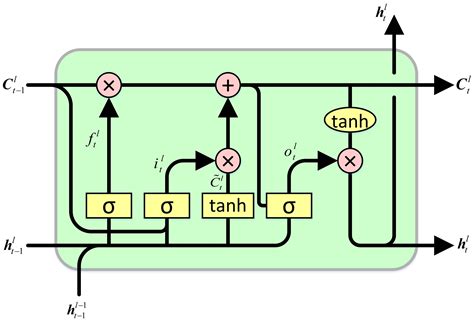
An LSTMCell computes four gates, then uses them to update the cell and hidden states. Each gate has the same dimension as the hidden state:
| Gate | Name | Activation | What It Does |
|---|---|---|---|
| \(i_t\) | Input gate | Sigmoid (0–1) | How much of the new candidate values to write into the cell |
| \(f_t\) | Forget gate | Sigmoid (0–1) | How much of the old cell state to keep (1 = remember everything, 0 = forget everything) |
| \(g_t\) | Cell gate | Tanh (-1 to 1) | The candidate new values to potentially add to the cell state |
| \(o_t\) | Output gate | Sigmoid (0–1) | How much of the cell state to expose as the hidden state output |
Notice the activation functions: three gates use sigmoid, but the cell gate uses tanh. This isn’t arbitrary. It reflects their different roles. The sigmoid gates (\(i_t, f_t, o_t\)) answer “how much?” questions: how much to write, how much to keep, how much to expose. Sigmoid squashes values to (0, 1), making each gate a dimmer switch that scales its input between “fully off” and “fully on.” The cell gate \(g_t\) answers a different question: “what values?” It proposes candidate content to write into the cell state. Tanh maps to (-1, 1), which is critical: it allows the cell state to both increase and decrease. If \(g_t\) used sigmoid (0, 1), the additive update \(i_t \odot g_t\) could only ever push the cell state upward, and it would grow without bound. Tanh lets the network write negative corrections, keeping the cell state centered and bounded.
A critical design choice is that the input gate and forget gate are completely independent: computed from separate weight matrices and biases, with nothing constraining them to sum to 1. The network is free to set both high, both low, or any combination.
Contrast this with the GRU (Gated Recurrent Unit), where the equivalent gates are complementary: a single update gate \(z_t\) weights new content by \(z_t\) and old content by \((1 - z_t)\), forcing a trade-off. The GRU is more parameter-efficient, but less expressive: it can only interpolate between “keep old” and “write new.”
The LSTM’s independence gives it four distinct operating modes:
| Forget \(f_t\) | Input \(i_t\) | Mode | Effect | When It’s Useful |
|---|---|---|---|---|
| \(\approx 1\) | \(\approx 1\) | Accumulate | Keep old state and write new info | Building up a running representation (e.g., accumulating features of a described entity) |
| \(\approx 0\) | \(\approx 1\) | Replace | Flush old state, write new info | Topic change or sentence boundary (start fresh with new content) |
| \(\approx 1\) | \(\approx 0\) | Preserve | Keep old state, ignore current input | Carrying information across irrelevant tokens (e.g., remembering subject across a parenthetical) |
| \(\approx 0\) | \(\approx 0\) | Reset | Forget old state and ignore input | Clearing a dimension that’s no longer needed |
The GRU can only express the diagonal of this table. This is why LSTMs tend to outperform GRUs on tasks requiring long-range memory: the accumulate mode lets information persist indefinitely while still absorbing new inputs, and the reset mode provides a clean mechanism for freeing capacity.
It’s tempting to think of gates as simple switches, but each gate is a learned pattern detector: analogous to how a CNN filter activates on specific visual patterns, a gate’s weight matrix learns to activate on specific contextual patterns in the input and hidden state. A CNN filter produces a high activation when the input patch matches its learned pattern; a gate weight matrix produces a high activation (close to 1 after sigmoid) when the combination of \(x_t\) and \(h_{t-1}\) matches its learned pattern. CNN filters detect spatial patterns in pixel neighborhoods; gate weights detect contextual patterns across the current token and sequence history.
Consider the forget gate: \(f_t = \sigma(W_{if} \cdot x_t + W_{hf} \cdot h_{t-1} + b_f)\). After training, specific rows of these weight matrices become specialized detectors:
This happens per dimension of the hidden state. The gate output is a vector, not a scalar: dimension 42 of the forget gate might be close to 0 (forget) while dimension 73 is close to 1 (keep), because each dimension stores different information and each gate dimension detects different patterns.
Even though we describe four separate gates, in practice we compute them all in one matrix multiplication by concatenating the four weight matrices into a single 4 * hidden_size matrix. We then split the result into four chunks. This is much faster because it replaces four small matmuls with one large one, better utilizing GPU parallelism and memory bandwidth.
With the conceptual foundation in place, let’s turn these equations into code. We’ll build two modules, LSTMCell (one time step) and LSTM (full sequences with multiple layers), verifying each against PyTorch’s official implementation.
LSTMCellWe implement two versions: a verbose one that makes every operation explicit (separate weight matrices for each gate), and a compact one using nn.Linear with the single-matrix trick. Both produce identical results. The compact version is what you’d use in practice.
import numpy as np
import torch
import torch.nn as nn
import torch.nn.functional as F## Long version
class LSTMCellNew(nn.Module):
def __init__(self, input_sz, hidden_sz, bias=True):
super().__init__()
self.weight_ih = nn.Parameter(torch.randn((input_sz, hidden_sz * 4)))
self.weight_hh = nn.Parameter(torch.randn((hidden_sz, hidden_sz * 4)))
self.bias_ih = nn.Parameter(torch.zeros(hidden_sz * 4))
self.bias_hh = nn.Parameter(torch.zeros(hidden_sz * 4))
def forward(self, x, h, c):
## B x hidden_sz
out = x @ self.weight_ih + h @ self.weight_hh + self.bias_ih + self.bias_hh
i, f, g, o = torch.split(out, 100, dim=-1)
i, f, o = torch.sigmoid(i), torch.sigmoid(f), torch.sigmoid(o)
g = torch.tanh(g)
c_t = f * c + i * g
h_t = o * torch.tanh(c_t)
return h_t, c_t## Short version utilizing linear layer module
class LSTMCellNew(nn.Module):
def __init__(self, input_sz, hidden_sz, bias=True):
super().__init__()
self.ih = nn.Linear(input_sz, hidden_sz * 4, bias=bias)
self.hh = nn.Linear(hidden_sz, hidden_sz * 4, bias=bias)
def forward(self, x, h, c):
out = self.ih(x) + self.hh(h)
i, f, g, o = torch.split(out, 100, dim=-1)
i, f, o = torch.sigmoid(i), torch.sigmoid(f), torch.sigmoid(o)
g = torch.tanh(g)
c_t = f * c + i * g
h_t = o * torch.tanh(c_t)
return h_t, c_tbatch_sz = 64
seq_len = 8
input_sz = 20
hidden_sz = 100
num_layers = 2X = torch.randn(seq_len, batch_sz, input_sz, dtype=torch.float32)
c_0 = torch.randn(num_layers, batch_sz, hidden_sz, dtype=torch.float32)
h_0 = torch.randn(num_layers, batch_sz, hidden_sz, dtype=torch.float32)pytorch_cell = nn.LSTMCell(input_sz, hidden_sz, bias=True)
(
pytorch_cell.weight_hh.shape,
pytorch_cell.weight_ih.shape,
pytorch_cell.bias_ih.shape,
pytorch_cell.bias_hh.shape,
)(torch.Size([400, 100]),
torch.Size([400, 20]),
torch.Size([400]),
torch.Size([400]))## h: B x hidden_sz
## c: B x hidden_sz
pytorch_h, pytorch_c = pytorch_cell(X[0], (h_0[0], c_0[0]))cell = LSTMCellNew(input_sz, hidden_sz)
## To make sure pytorch and our implementation both
## have the same weights so we can compare them
cell.ih.weight.data = pytorch_cell.weight_ih.data
cell.hh.weight.data = pytorch_cell.weight_hh.data
cell.ih.bias.data = pytorch_cell.bias_ih.data
cell.hh.bias.data = pytorch_cell.bias_hh.datah_t, c_t = cell(X[0], h_0[0], c_0[0])print(
np.linalg.norm(pytorch_h.detach().numpy() - h_t.detach().numpy()),
np.linalg.norm(pytorch_c.detach().numpy() - c_t.detach().numpy()),
)0.0 0.0LSTMWith LSTMCell verified, let’s build the full LSTM module that handles entire sequences and optionally stacks multiple layers.
There are several important design decisions in a production LSTM implementation:
Memory layout: sequence-first (T × B × D). We use the sequence length as the first dimension instead of batch-first. Why? We iterate over time steps in the inner loop, and we want each x[t] to be a contiguous slice of memory. If batch were first, each time step’s data would be non-contiguous, requiring a copy on every iteration.
If you pass batch-first tensors (B × T × D) to an LSTM that expects sequence-first, it will still “work”, but each time step access triggers an implicit copy because the memory isn’t contiguous along the time dimension. This can silently slow down training. PyTorch’s nn.LSTM has a batch_first flag that handles the transpose for you, but internally it still processes sequence-first.
Truncated Backpropagation Through Time (TBPTT). Since weights are shared across all time steps within a layer, backpropagating through very long sequences causes severe vanishing/exploding gradients and extreme memory usage (all intermediate activations must be stored). The standard solution: detach the hidden and cell states from the computation graph after each batch. Gradients can flow within a batch’s time steps but not across batch boundaries.
Multi-layer stacking. We can stack LSTMs by feeding the hidden state output of layer \(l\) as the input to layer \(l+1\). Each layer has its own LSTMCell with independent weights. The first layer’s cell takes input of size input_sz; all subsequent layers take input of size hidden_sz. This increases model capacity: deeper layers can learn more abstract representations.
Layer iteration order. With multiple layers, there are two valid iteration orders: (1) iterate all time steps for layer 0, then all time steps for layer 1, etc., or (2) at each time step, iterate through all layers before moving to the next time step. Our implementation uses option (1), which is simpler and matches PyTorch’s behavior.
Handling variable-length sequences. Not all sequences have the same length. Two approaches:
pack_padded_sequence and pad_packed_sequence utilities for this.class LSTMNew(nn.Module):
def __init__(self, input_sz, hidden_sz, num_layers=1):
super().__init__()
self.num_layers = num_layers
self.hidden_sz = hidden_sz
self.cells = nn.ModuleList(
[
LSTMCellNew(input_sz, hidden_sz)
if i == 0
else LSTMCellNew(hidden_sz, hidden_sz)
for i in range(self.num_layers)
]
)
def forward(self, x, h_t, c_t):
## x : T x B x hidden_sz
## h_t: num_layers x B x hidden_sz
## c_t: num_layers x B x hidden_sz
T, B, _ = x.shape
H = torch.zeros(T, B, self.hidden_sz)
for i, cell in enumerate(self.cells):
h, c = h_t[i], c_t[i]
if i > 0:
x = H
for t in range(T):
h, c = cell(x[t], h, c)
H[t] = h
## last hidden state for each layer
h_t[i], c_t[i] = h, c
## Truncated BPTT
return H, (h_t.detach(), c_t.detach())pytorch_lstm = nn.LSTM(input_sz, hidden_sz, num_layers=num_layers)
pytorch_H, (pytorch_h, pytorch_c) = pytorch_lstm(X, (h_0, c_0))lstm = LSTMNew(input_sz, hidden_sz, num_layers=num_layers)
for i in range(num_layers):
lstm.cells[i].ih.weight.data = getattr(pytorch_lstm, f"weight_ih_l{i}").data
lstm.cells[i].hh.weight.data = getattr(pytorch_lstm, f"weight_hh_l{i}").data
lstm.cells[i].ih.bias.data = getattr(pytorch_lstm, f"bias_ih_l{i}").data
lstm.cells[i].hh.bias.data = getattr(pytorch_lstm, f"bias_hh_l{i}").data
H, (h_t, c_t) = lstm(X, h_0, c_0)print(
np.linalg.norm(pytorch_H.detach().numpy() - H.detach().numpy()),
np.linalg.norm(pytorch_h.detach().numpy() - h_t.detach().numpy()),
np.linalg.norm(pytorch_c.detach().numpy() - c_t.detach().numpy()),
)0.0 0.0 0.0LSTMs were the dominant architecture for sequence modeling in NLP for years, powering machine translation, text classification, language modeling, and speech recognition before Transformers took over. In this post, we implemented both LSTMCell and a multi-layer LSTM from scratch, verified them against PyTorch’s official implementation, and discussed the performance decisions that go into a production implementation.
LSTMs solve vanishing gradients through additive cell state updates. The forget gate can stay close to 1, allowing gradients to flow through many time steps without exponential decay. This is fundamentally different from vanilla RNNs, where the hidden state is completely overwritten at each step.
Four gates, one matrix multiplication. The input, forget, cell, and output gates are computed together in a single fused operation, then split, a practical optimization that significantly improves throughput by better utilizing hardware parallelism.
Sequential processing is the fundamental bottleneck. The output at time \(t\) depends on the hidden state from \(t-1\), making parallelization across time steps impossible. This is the limitation that motivated the Transformer’s self-attention mechanism.
Truncated BPTT is essential for long sequences. Detaching hidden states between batches prevents gradient computation from spanning the entire sequence, reducing both memory usage and gradient instability.
Memory layout matters. Using sequence-first tensors (T × B × D) ensures contiguous memory access at each time step, avoiding hidden performance penalties from implicit copies.
While Transformers have largely replaced LSTMs for most NLP tasks, understanding LSTMs remains valuable. They’re still used in streaming/online settings where you process one token at a time, in resource-constrained environments where the \(O(n^2)\) attention cost is prohibitive, and as components in hybrid architectures. More importantly, the concepts (gating, cell states, truncated BPTT) appear in many modern architectures in different forms.